ecpEnergyTwinAnalytics
Energy Twin Analytics machine learning extension for energy data analysis
Registered StackHub users may elect to receive email notifications whenever a new package version is released or a comment is posted on the forum.
There are 0 watchers.
Welcome to the Energy Twin (ET) extension for SkySpark. Energy Twin is a machine learning-based SkySpark extension for energy data analysis and prediction.
Energy Twin libraries available on StackHub:
See the ET website for case studies and more information: Energy Twin webpage.
Welcome to the Energy Twin (ET) extension for SkySpark. Energy Twin is a machine-learning-based SkySpark extension for energy data analysis. Using the Energy Twin extension, you can predict energy consumption. ET is designed to efficiently monitor multiple buildings using artificial intelligence to identify problems and reveal future energy consumption savings and optimization potential. Detailed information about the mathematical model used by ET and adherence with M&V guidelines can be found on ET website.
Once you have logged into your SkySpark account, ET icons can be seen in the main menu.
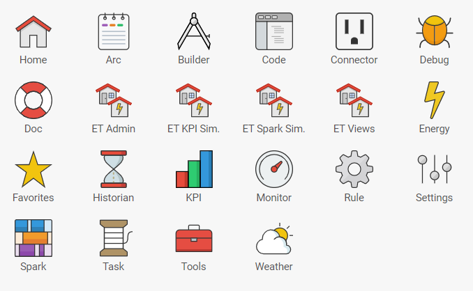
To create or train a new model, select the ET Admin icon in the main menu.
After opening ET Admin, you get to the Administration tab. There are other tabs available in the tab menu - Training and Manual.
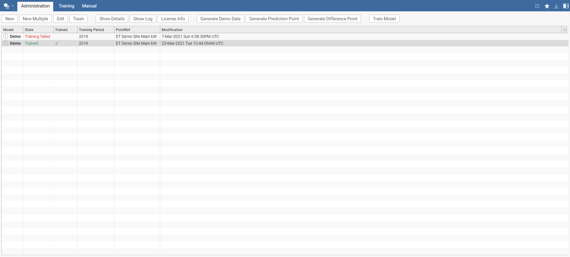
In the Administration tab, you can see an overview of your models once you have created them. Before you create your first model, this overview will be empty.
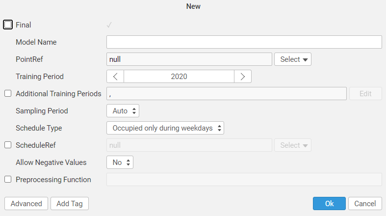
To create a new model, select New in the menu toolbar. A pop-up window appears, where you specify your new model's name, training period, on which point it will be trained, and any other additional information such as schedule, etc. It is also possible to add an additional training period.
For Sampling Period, there are four options:
While selecting Schedule Type, there are four options:
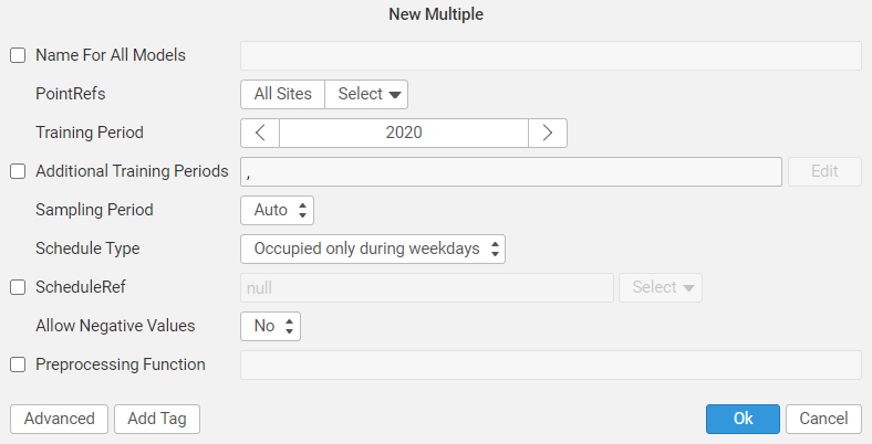
Multiple models can also be created at the same time by selecting the option New Multiple in the menu toolbar.
After creating your model(s), a list of your models, status, and additional information such as training date, modification date, and point location appears. Also, new options will be available in the toolbar menu:
Note that there can be multiple models linked to one point. In such a case, you can mark one of the models as "Final". The model marked as Final will be used for sparks and other applications where user cannot specify the model explicitly. After selecting Train model, the model will be added to the training queue. The training process can be observed in the Training tab.
In the Training tab, you can see an overview and status of your trained models. You can choose to retrain a model or to delete them from the training overview.
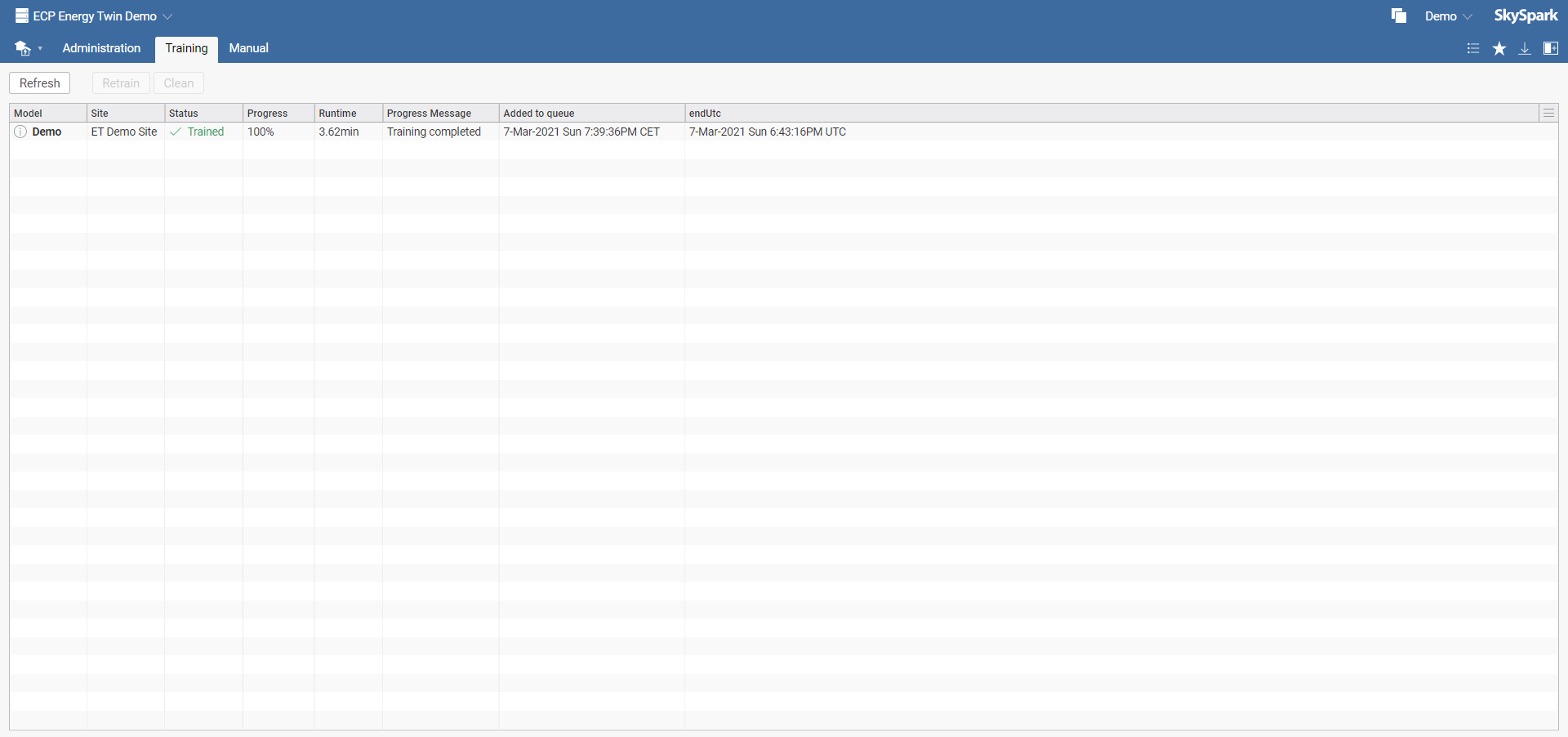
Disclaimer: Selecting Clean in the toolbar menu won't delete the model. It will only remove the information about training from the training overview. To delete a model, select Trash in the Administration tab.
For help or more information, select the tab Manual to see this document.
For successful training, a model must include information about the weather, point location, and schedule. If one of these three parameters is missing, the model cannot be trained, and you have to revise your point. Weather information is provided by SkySpark automatically using built-in toWeather function. If there is a timezone difference between schedule or weather and point location, the model cannot be trained.
The rule of thumb is to choose one year identification period. Selecting suitable identification is very important. For more information on this topic, see M&V guidelines - section Identification period selection.
There are buit-in preprocessing fucntions as well as user defined preprocessing functions. User can implement own data preprocessing used for data identification (e.g. specific outliers removal). User defined preprocessing can also be used for narrowing the identification period (e.g., leave out every Sunday). Data Preprocessing consists of three parts:
(data, opts) => do
  // Minimum value
  if(opts.has("minVal")) do
    data = data.findAll(x => x["meas"] >= opts->minVal)
  end
  // Maximum value
  if(opts.has("maxVal")) do
    data = data.findAll(x => x["meas"] <= opts->maxVal)
  end
  return data
end(data, allowNegativeValues) => do
data = data.findAll x => do
x["meas"] != null and x["meas"] != nan() and x["meas"] != na() and not isNaN(x["meas"]) and
x["ts"] != null and x["ts"] != nan() and x["ts"] != na() and not isNaN(x["ts"])
end
if(not allowNegativeValues) do
data = data.findAll(x => x["meas"] >= 0)
end
return data
endAfter selecting ET Views icon in the main menu, you get to the Load Profile tab. There are other tabs available in the tab menu - Modeled vs. Measured, Monthly Differences, Sparks Viewer, and Report Exporter.
Load Profile
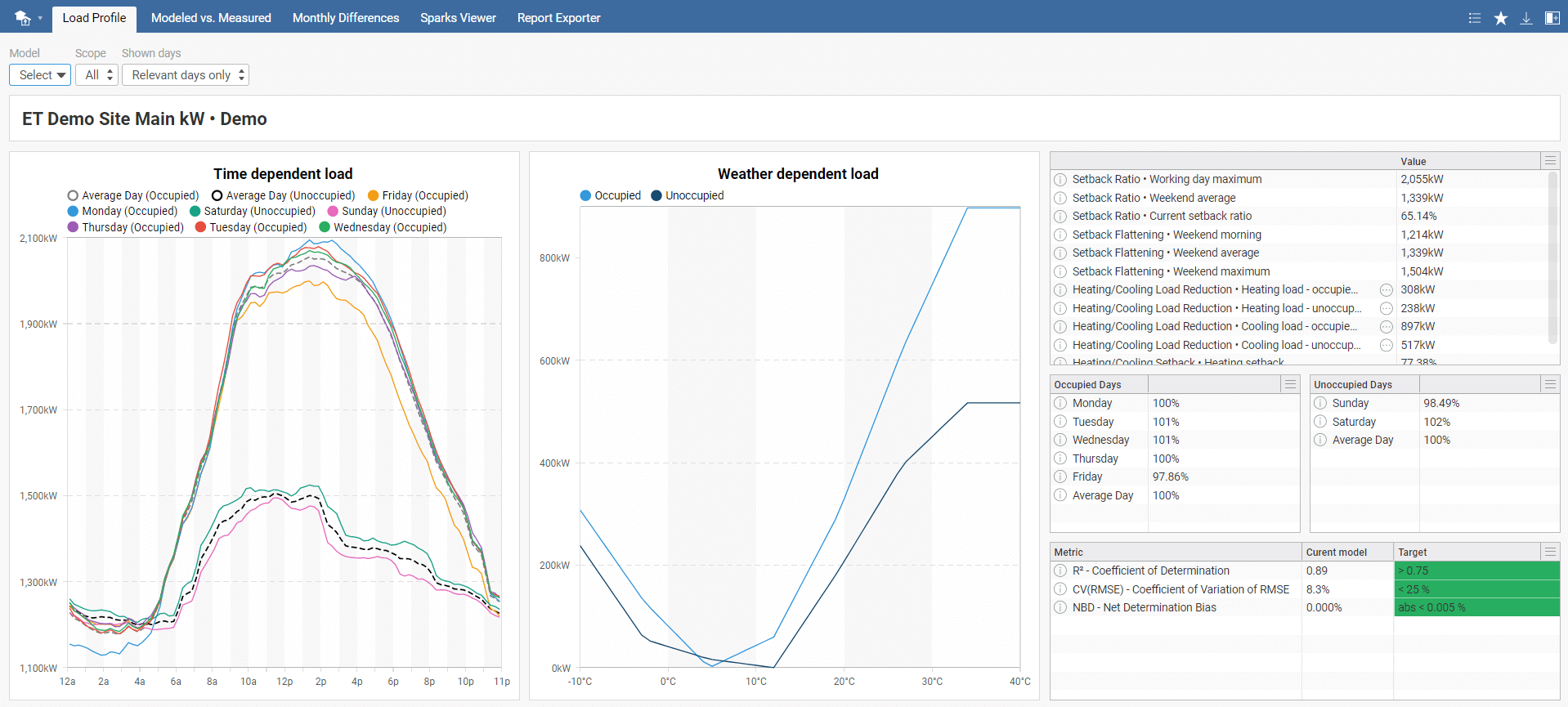
In the tab toolbar menu, there are three options: Model, Scope, and Shown days. Start by selecting your model. You can choose to show only occupied or unoccupied days in the scope option, and in shown days, you can show either relevant days (i.e. weekdays with sufficient amout of data in the training period) or all days. All days option contains all days in occupied and unoccupied mode.
On the right side, there are overview charts of all KPIs and percentage distribution of energy consumption compared to an average day. The last table shows used metrics and their values with recommended targets.
Disclaimer: Please note that the distribution of the load between weather dependent and time dependent is only informative. With an unbalanced dataset, incorrect data load distribution is possible. See the weather dependent profile for both occupied and unoccupied days. If it doesn't meet your expectations, be careful while interpreting the results. For more information, see the ET Model Description document at https://et.mervis.info/wp-content/uploads/2021/04/ET_Model_Description.pdf .
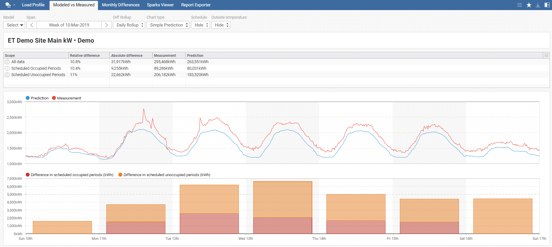
Modeled vs. Measured
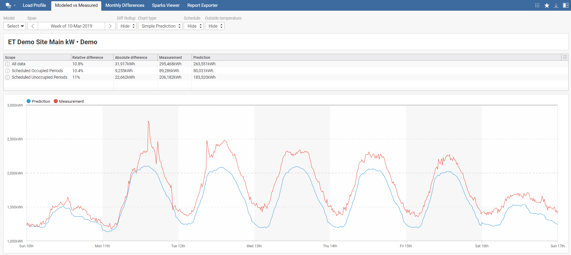
After selecting Modeled vs. Measured, a new tab toolbar menu appears with the following options: Model, Span, Diff Rollup, Chart type, Schedule, and Outside temperature. First, select your model and required time span. Diff Rollup option either hides or generates Daily Rollup, Weekly Rollup, or Monthly Rollup. It is used for determining the difference in predicted and measured energy consumption. In other words, to see if selected model predictions correspond to measured energy consumption.
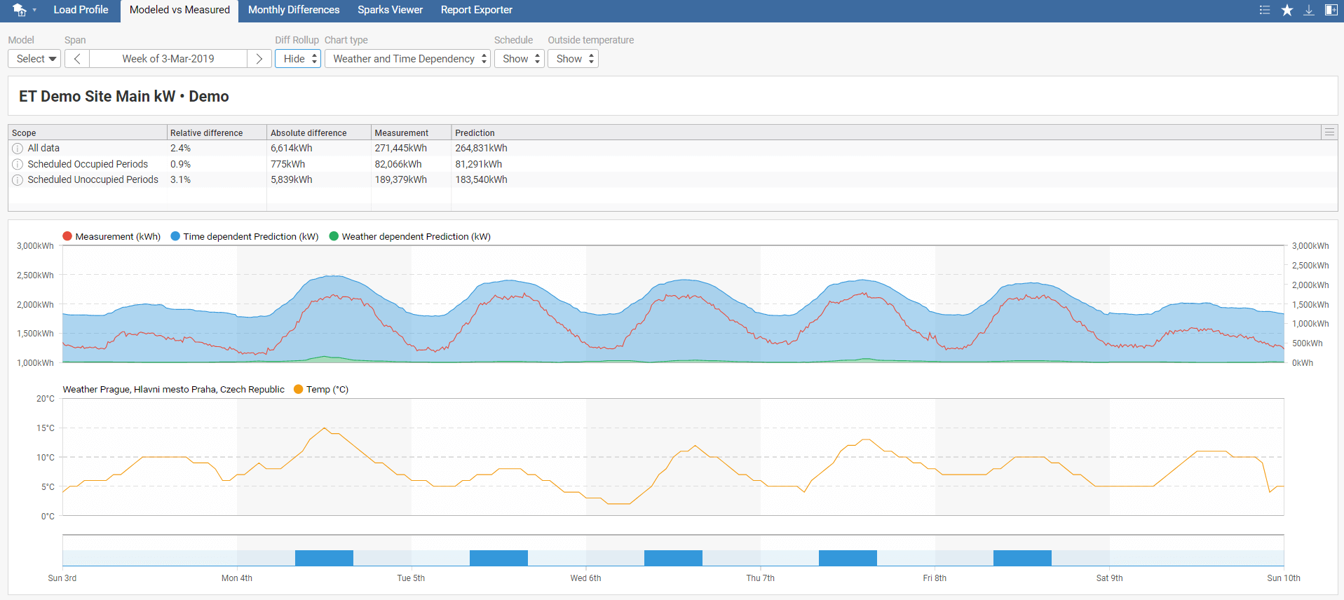
You can modify the output graph by changing the Chart type to confidence intervals or time and weather dependency. Also, it is possible to show/hide the schedule and outside temperature.
Disclaimer: Please note that the distribution of the load between weather dependent and time dependent is only informative. With an unbalanced dataset, incorrect data load distribution is possible. See the weather dependent profile for both occupied and unoccupied days. If it doesn't meet your expectations, be careful while interpreting the results. For more information, see the ET Model Description document at https://et.mervis.info/wp-content/uploads/2021/04/ET_Model_Description.pdf .
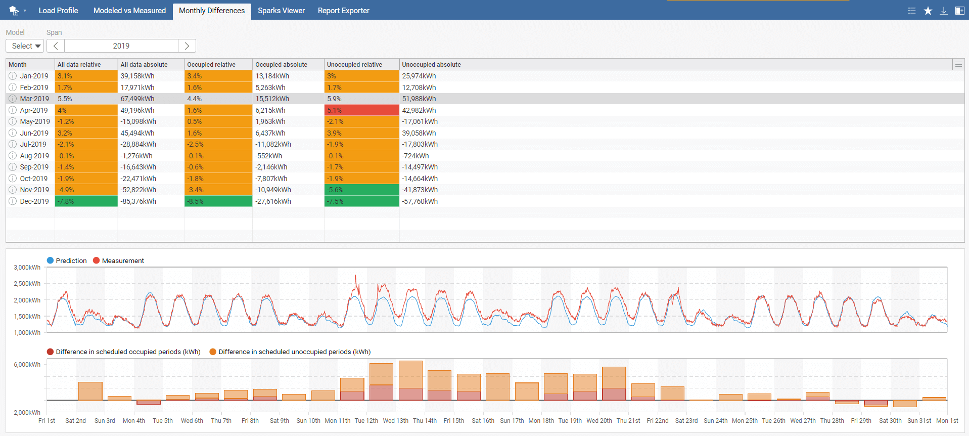
The Monthly Differences tab generates an overview table over the selected year. You should pay attention to the values with the red background. After clicking on a row detailed monthly chart will appear.
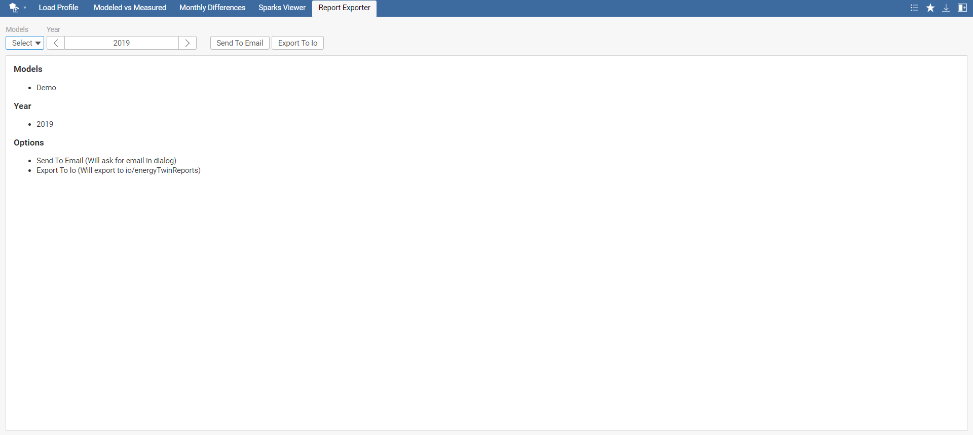
Report Exporter tab allows you to generate a yearly PDF report of your model and send it via e-mail or export to Io.
After selecting ET Spark Sim., you get to the Absolute Value Deviation tab. There are other available tabs in the tab menu - Relative Value Deviation, Statistical Deviation, and Integral Deviation.
Sparks are tests conducted on points for suspicious behavior detection and fault detection. To access sparks, select ET views in the main menu. Apart from sparks themselves, the tools Sparks Simulator and Sparks Viewer are described in this section.
Absolute Value Deviation spark detects when the difference between measured and predicted energy consumption exceeds the selected threshold value. Returned cost is the sum of the difference between measured and predicted energy consumption over the intervals when the spark is active. Note that it is possible use negative thresholds, e.g., when the predicted energy consumption was bigger than real measurement.
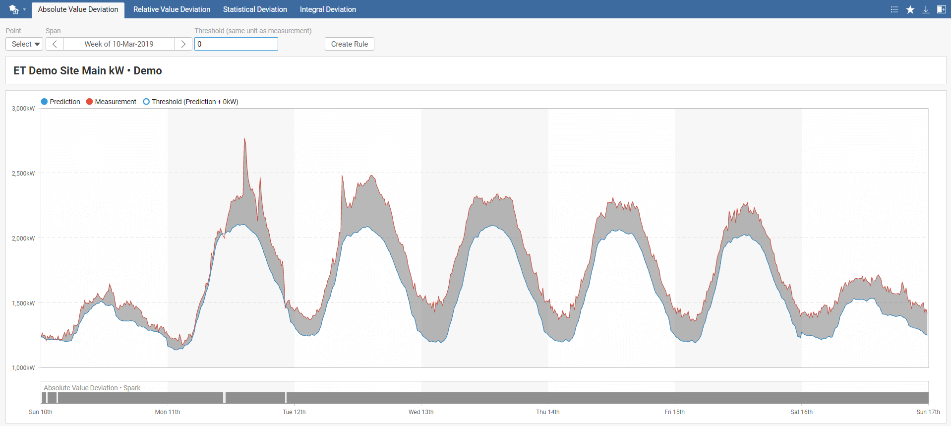

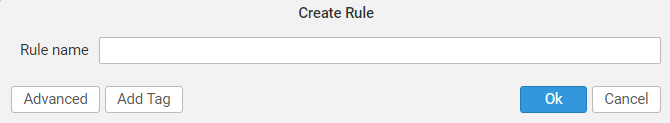
In the Absolute Value Deviation toolbar menu, select your model, required time span, and threshold. The default threshold value is set to 0. You can also instantly create a new rule by clicking on Create Rule, which you can name in the pop-up window. This rule will be added to Rules in the main menu.
Relative Value Deviation spark detects when the difference between measured and predicted energy consumption exceeds the selected threshold value. Threshold is defined relatively to the prediction.
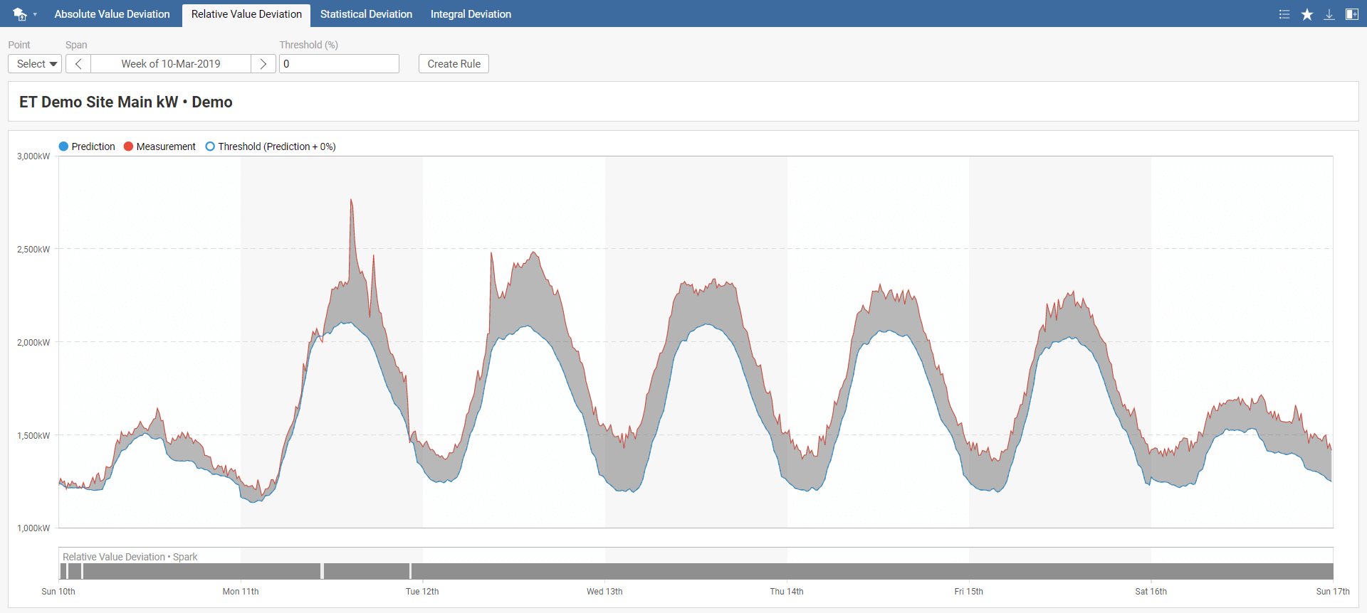
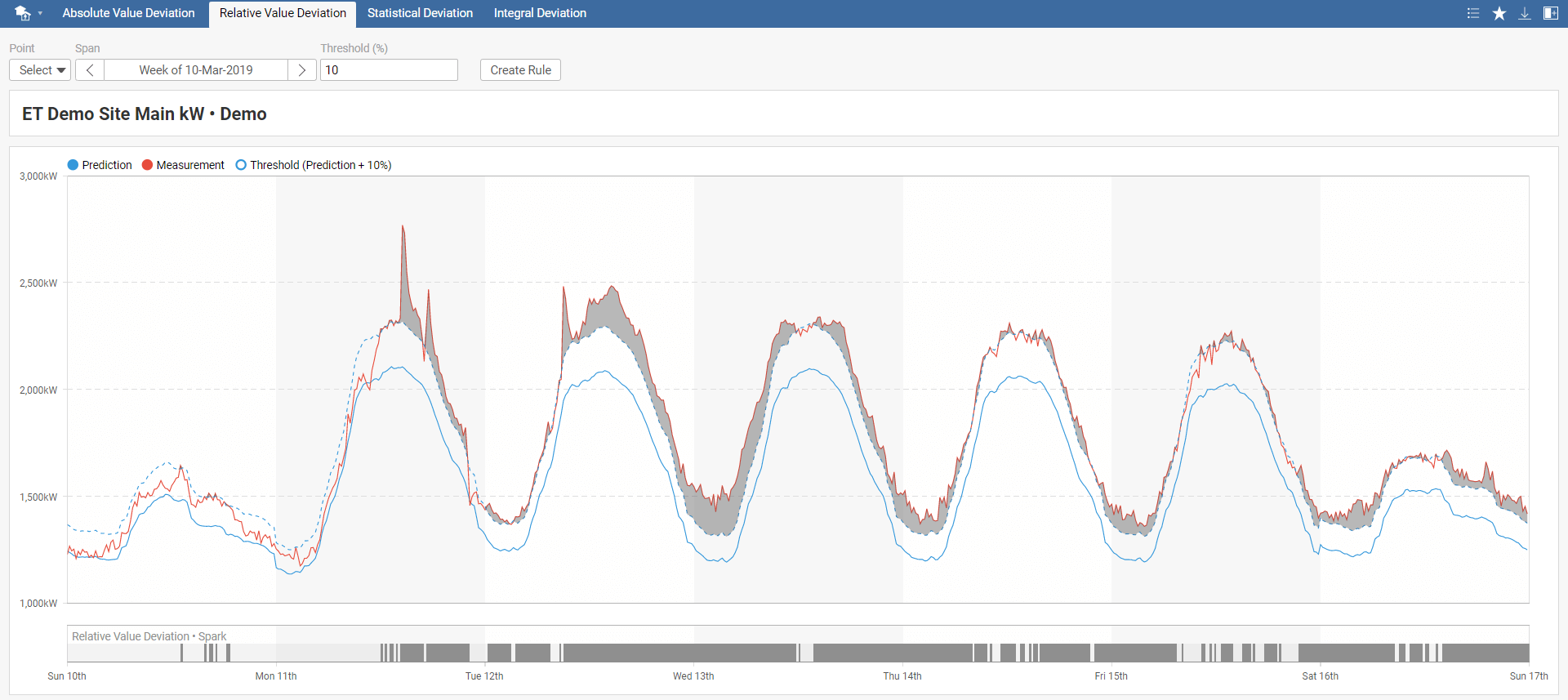
In the Relative Value Deviation toolbar menu, select your model, required time span, and threshold. The default threshold value is set to 0. You can also instantly create a new rule by clicking on Create Rule, which you can name in the pop-up window. This rule will be added to Rules in the main menu.
Statistical Deviation spark evaluates the difference between measured and predicted energy consumption exceeds confidence interval multiplied by models' standard deviation. The selected threshold value can be negative, in which case we detect when measured energy consumption is lower than the confidence interval multiplied by selected the threshold value compared to predicted energy consumption. Recommended values are +/- 1, +/- 3, and +/- 10, where 1 is the most sensitive.
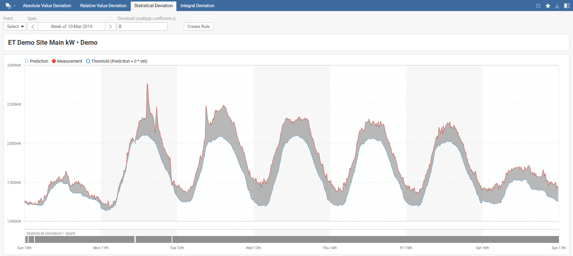
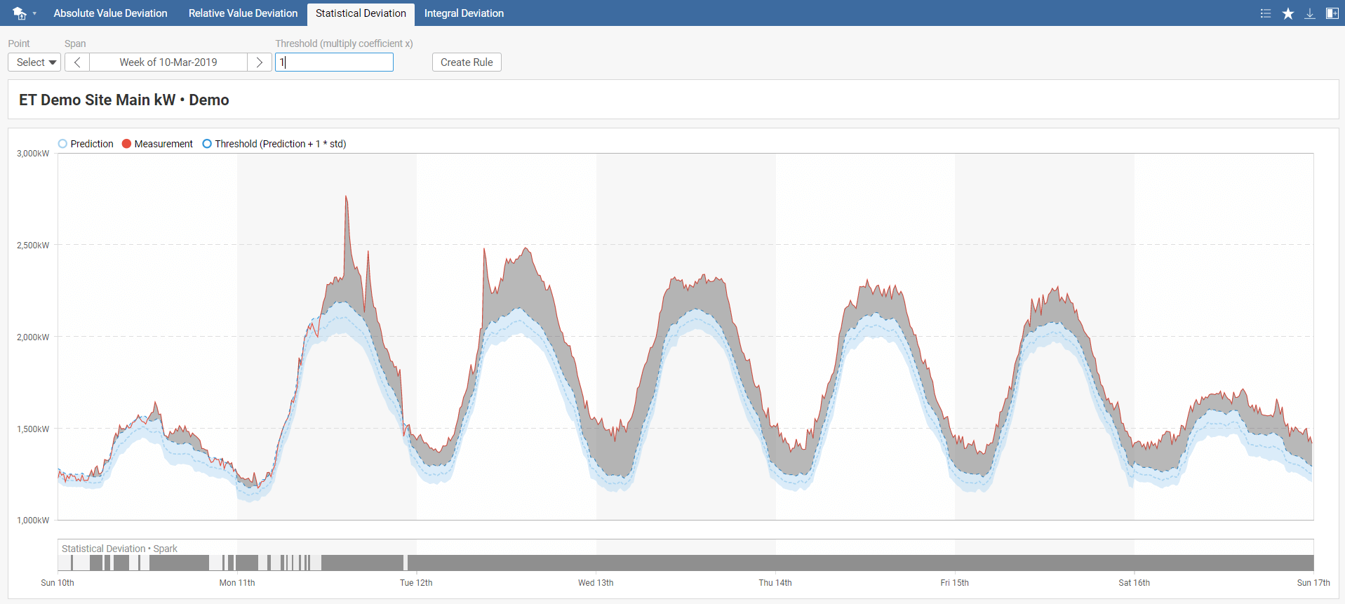
In the Statistical Deviation toolbar menu, select your model, required time span, and threshold. The default value of the threshold is set to 0. You can also instantly create a new rule by clicking on Create Rule, which you can name in the pop-up window. This rule will be added to Rules in the main menu.
This spark detects when the sum of the difference between measured and predicted energy consumption is greater than the selected threshold value. There are two possible scenarios for using this spark. You can either evaluate each day separately or detect trends over a long period. Daily evaluation is typically used for detecting significant deviations from predictions usually caused by faults. Assessment over a more extended period shows gradual system efficiency degradation.
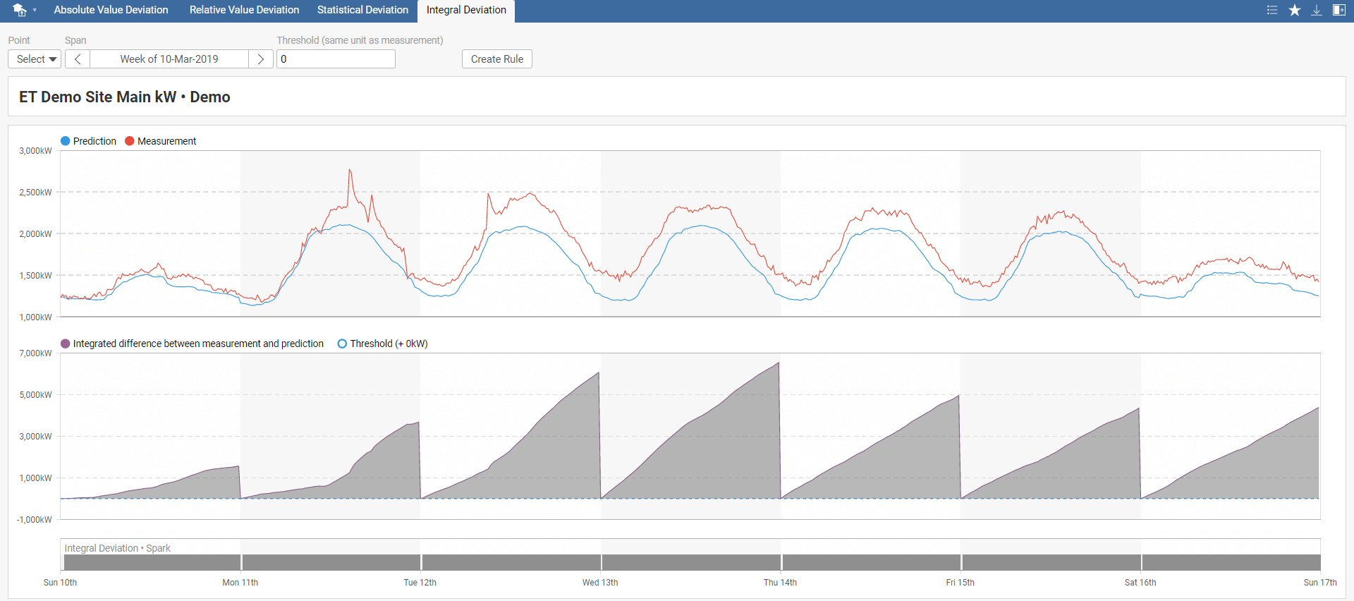
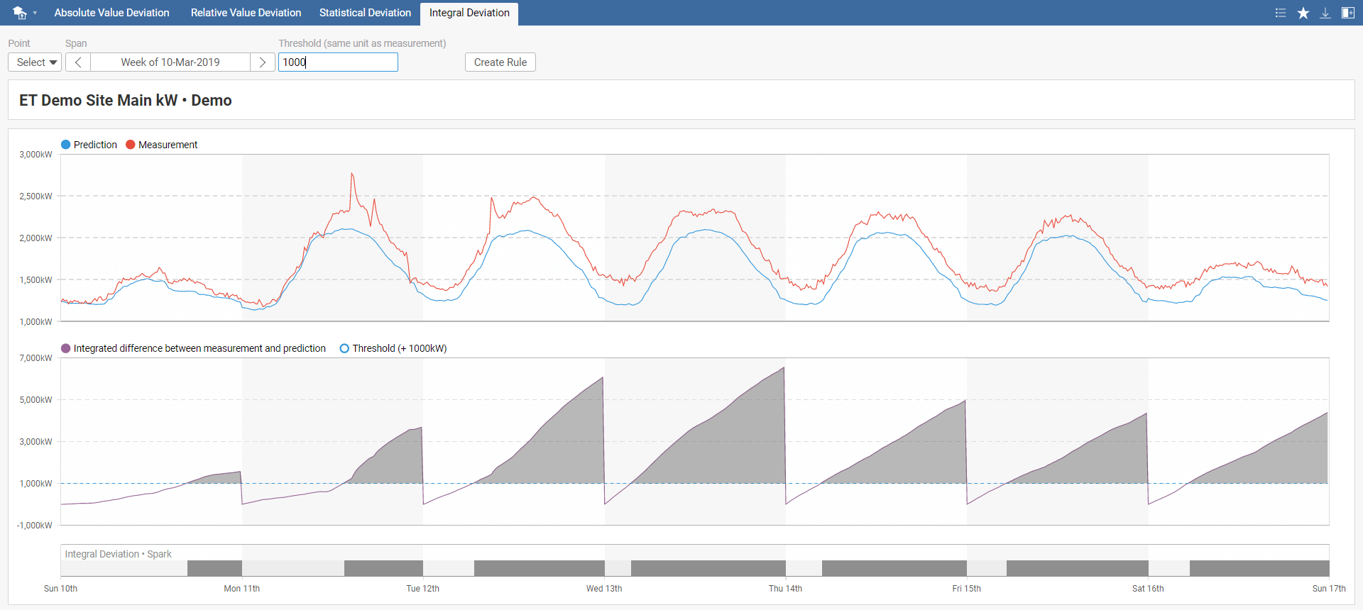
In the Integral Deviation toolbar menu, select your model, required time span, and threshold. The default value of the threshold is set to 0. You can also instantly create a new rule by clicking on Create Rule, which you can name in the pop-up window. This rule will be added to Rules in the main menu.
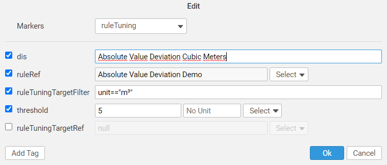
Tuning framework allows user to tune their rules as can be seen in the following example, where the threshold value changes according to units. Rules can be also tuned depending on which building it is etc. This can be done in the SkySpark's app Rules.
After selecting ET KPI Sim. icon in the main menu, you get to the Setback Ratio tab. There are other tabs available in the tab menu - Setback Flattening, Saturday Sunday Equalization, Heating/Cooling Setback, and Heating/Cooling Load Reduction.
Energy Twin uses the KPI system from SkySpark, the values are calculated in advance which allows quick viewing of the results. KPIs are suitable for If-Then scenarios simulation.
The Setback Ratio expresses the average power ratio during an average weekend day and maximum power during an average working day. This KPI is suitable for buildings with regular weekend setbacks such as offices or schools and evaluates differences during unoccupied days only.
Setback Ratio interpretation:
What to do: First, check schedules of major technologies such as AHUs or FCUs. Are their setbacks set correctly? Alternatively, detailed measurement of electrical consumption outside office hours should be performed (e.g., using a power clamp meter).
When to ignore: Any building without a setback, typically hospitals, shopping malls, hotels, etc. Special technologies such as servers can cause high values of setback ratio.
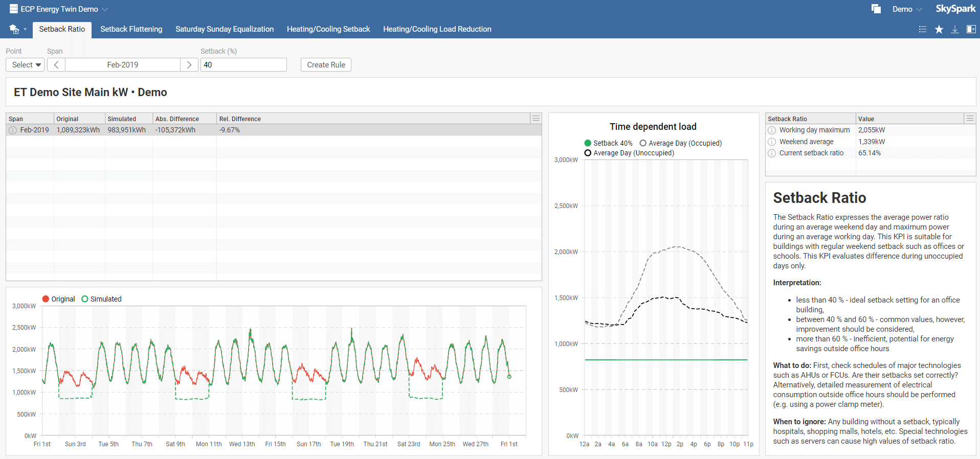
In the Setback Ratio toolbar menu, select your model, required time span, and setback. The default setback value is set to 40. You can also instantly create a new rule by clicking on Create Rule, which you can name in the pop-up window. This rule will be added to Rules in the main menu.
Disclaimer: Please note that the distribution of the load between weather dependent and time dependent is only informative. With an unbalanced dataset, incorrect data load distribution is possible. See the weather dependent profile for both occupied and unoccupied days. If it doesn't meet your expectations, be careful while interpreting the results. For more information, see the ET Model Description document at https://et.mervis.info/wp-content/uploads/2021/04/ET_Model_Description.pdf .
The Setback Flattening estimates the amount of possibly saved energy if there is no increase in energy consumption during unoccupied days (i.e., energy consumption will be the same as in the early morning). This KPI evaluates differences during unoccupied days only.
Setback Flattening interpretation: The KPI expresses the energy-saving potential estimate. The energy-saving potential estimate provides a helpful guideline for deciding whether a detailed technical investigation is worth the effort.
What to do: Check schedules of appliances that can cause an increase in energy consumption during unoccupied days in the daytime. Focus on appliances turned on after 5 am, i.e., it does not run non-stop.
When to ignore: Any building without a setback, typically hospitals, shopping malls, hotels, etc. Also, buildings with combined offices and retail could have increased consumption, especially on Saturdays.
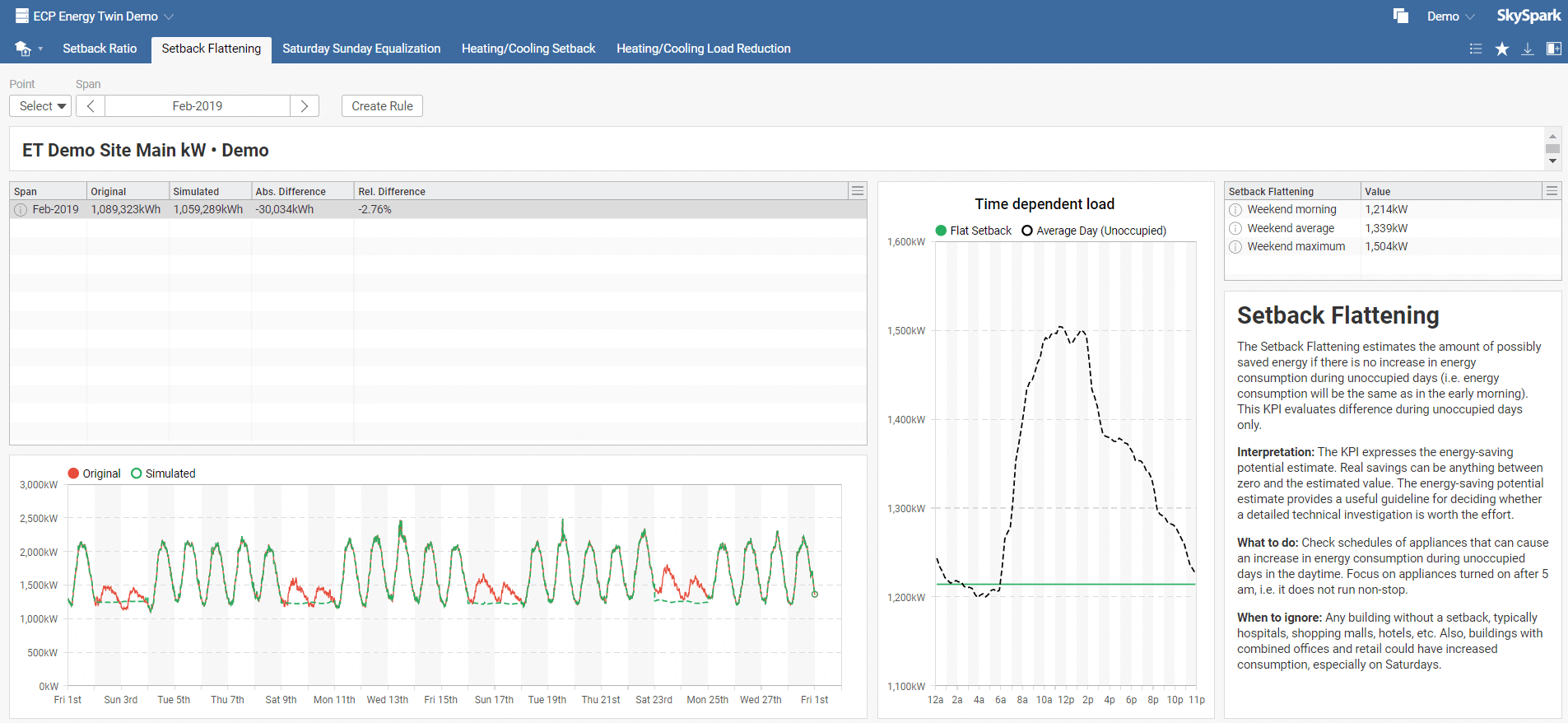
In the Setback Flattening toolbar menu, select your model and required time span. You can also instantly create a new rule by clicking on Create Rule, which you can name in the pop-up window. This rule will be added to Rules in the main menu.
Applicable to buildings with expected same weekend setbacks for Saturday and Sunday. This KPI estimates energy-saving potential if both days have the same profile equal to the lower of these two. Typically, how much energy can be saved if Saturday will be the same as Sunday. This KPI evaluates differences during unoccupied days only.
Saturday Sunday Equalization interpretation: The KPI expresses the energy-saving potential estimate. Actual savings can be anything between zero and the estimated value. The energy-saving potential estimate provides a helpful guideline for deciding whether a detailed technical investigation is worth the effort.
What to do: Check the difference between Saturday and Sunday appliance schedules.
When to ignore: Any building with the expected difference between Saturday and Sunday regime, e.g., a big office building with some small shops open during Saturday morning.
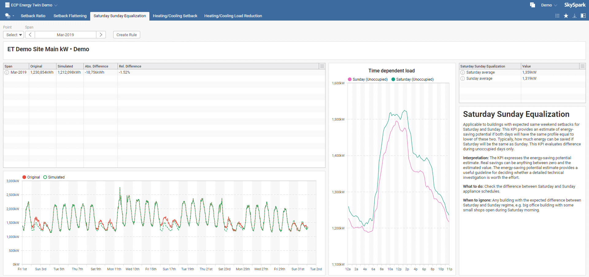
In the Saturday Sunday Equalization toolbar menu, select your model and required time span. You can also instantly create a new rule by clicking on Create Rule, which you can name in the pop-up window. This rule will be added to Rules in the main menu.
This KPI allows the simulation of heating and cooling setback. The heating (cooling) load during unoccupied days is expressed as a percentage of the heating (cooling) load during occupied days. This KPI addresses the common problem of office buildings when there is no cooling setback during weekends. It estimates energy savings that can be achieved by cooling setback (e.g., 50 % setback). This KPI evaluates differences during unoccupied days only.
Heating/Cooling Setback interpretation: Measurement is compared with a prediction with changed parameters (e.g., 50 % cooling setback).
What to do: This KPI provides an estimate of saving potential. Actual savings can be anything between zero and the estimated value. The energy-saving potential estimate offers a helpful guideline for deciding whether a detailed technical investigation is worth the effort.
When to ignore: Any building without a setback, typically hospitals, shopping malls, hotels, etc. Also, pay attention to the shape of the weather dependent load. Typically it has \_/ shape (heating and cooling), \_ shape (heating only), or _/ shape (cooling only). If the shape does not meet the expectations, the KPI result will probably be misleading. In that case, try to re-identify the model using more extensive data sets or exclude outliers from the training data period.
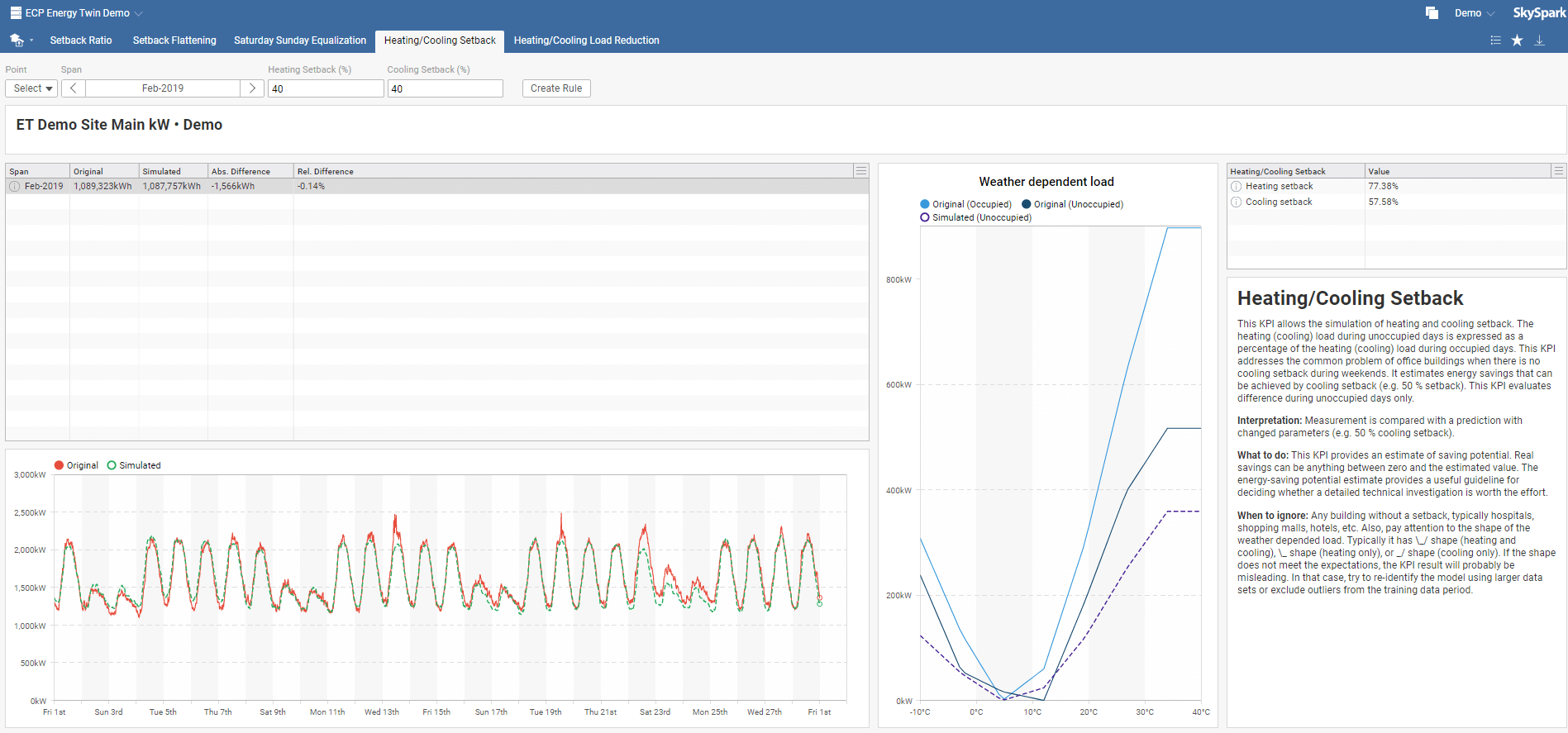
In the Heating/Cooling Setback toolbar menu, select your model, required time span, heating occupied load, heating unoccupied load, cooling occupied load, and cooling unoccupied load. Default setback values are set to 100. You can also instantly create a new rule by clicking on Create Rule, which you can name in the pop-up window. This rule will be added to Rules in the main menu.
Disclaimer: Please note that the distribution of the load between weather dependent and time dependent is only informative. With an unbalanced dataset, incorrect data load distribution is possible. See the weather dependent profile for both occupied and unoccupied days. If it doesn't meet your expectations, be careful while interpreting the results. For more information, see the ET Model Description document at https://et.mervis.info/wp-content/uploads/2021/04/ET_Model_Description.pdf .
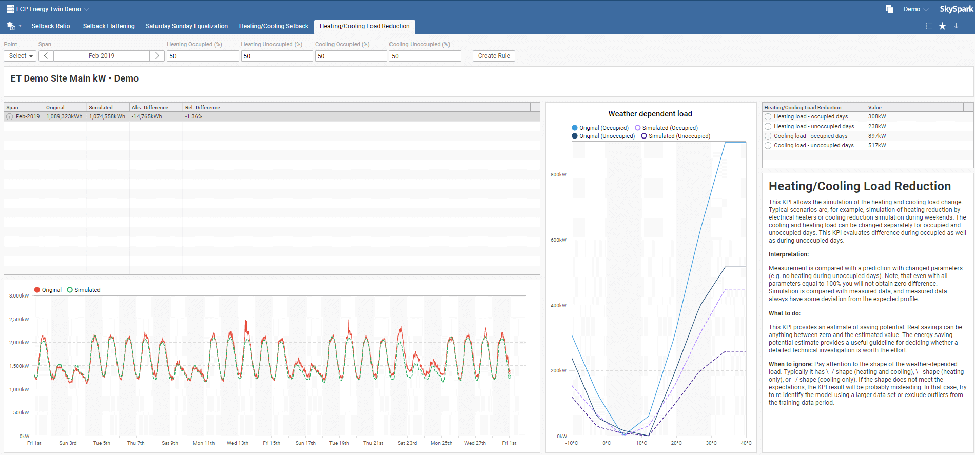
This KPI allows the simulation of the heating and cooling load change. Typical scenarios are, for example, simulation of heating reduction by electrical heaters or cooling reduction simulation during weekends. The cooling and heating load can be changed separately for occupied and unoccupied days. This KPI evaluates differences during occupied as well as during unoccupied days.
Heating/Cooling Load Reduction interpretation: Measurement is compared with a prediction with changed parameters (e.g., no heating during unoccupied days). Note, that even with all parameters equal to 100 %, you will not obtain zero difference. Simulation is compared with measured data, and measured data always have some deviation from the expected profile.
What to do: This KPI provides an estimate of saving potential. Actual savings can be anything between zero and the estimated value. The energy-saving potential estimate offers a helpful guideline for deciding whether a detailed technical investigation is worth the effort.
When to ignore: Pay attention to the shape of the weather-depended load. Typically it has \_/ shape (heating and cooling), \_ shape (heating only), or _/ shape (cooling only). If the shape does not meet the expectations, the KPI result will probably be misleading. In that case, try to re-identify the model using a more extensive data set or exclude outliers from the training data period.
In the Heating/Cooling Setback toolbar menu, select your model, required time span, heating setback, and cooling setback. Default setback values are set to 100. You can also instantly create a new rule by clicking on Create Rule, which you can name in the pop-up window. This rule will be added to Rules in the main menu.
Disclaimer: Please note that the distribution of the load between weather dependent and time dependent is only informative. With an unbalanced dataset, incorrect data load distribution is possible. See the weather dependent profile for both occupied and unoccupied days. If it doesn't meet your expectations, be careful while interpreting the results. For more information, see the ET Model Description document at https://et.mervis.info/wp-content/uploads/2021/04/ET_Model_Description.pdf .
API Functions are Axon functions that are available for users. Only a brief description will be provided, for more information, see functions' documentation.
This function calculates a prediction of the given model. Occupancy and weather data are loaded using weather corresponding to the given point and its schedule. Prediction is composed of mean value and standard deviation.
Example: etModelPredict(read(etModel and trained), 2019-01)
This function returns a trained model for the given point.
Example: metGetModelForPoint(read(point))
This function returns predicted energy consumption divided into a time-dependent and weather-dependent load.
Example: metModelPredict(read(etModel and trained), 2019-01)
This function attempts to fix model recods. It adds required tags if they are missing or corrupted. Model's parameter is optional, when null - it will read all models.
Example: etFixModels()
This function will create new model.
Example: etModelCreate("my model 2", read(point)->id, 2019)
Example: etModelCreate("my model 2", read(point)->id, 2019, {scheduleType:"occupiedEveryDay"})
This function will add models to training queue.
Example: etModelTrain([@modelId1, @modelId2, readAll(etModel)[3])
Example: etModelTrain(@modelId)
This function generates demo site with equip and point, weather, and trained model. If there are any records in project with tag etDemogen, a new demo site won't be produced.
Example: etDemogen()
Function ready to be used as a hisFunc. This function returns model prediction. Tag measurementPointRef is has to be defind on a point that uses this hisFunc.
Function ready to be used as a hisFunc. This function returns diffence between measured and predicted values. Tag measurementPointRef is has to be defind on a point that uses this hisFunc.
Q : The model was not trained. Why?
A : Go to the Training view and see the message in the Progress Message column. If this does not help, you can also see more info by clicking on the information icon.
Q : Identified model does not fit the measurement.
A : First, check the Schedule Type settings and linked Weather station. Then see data from the identification period - are there any outliers? Are there constant data? Is there any non-representative time period? If you answer yes to any of these questions, you should pay attention to data preprocessing and identification period selection (see Additional periods option). Lastly, think about the building schedule and note that the model is linear. In other words, it cannot model non-linearities. An example of such non-linearity could be a significant change in building usage or a manual start of some energy-intensive appliance.
Q : My data are confidential. Are they send to the Internet during the identification or prediction process?
A : No. Everything is calculated using standard SkySpark libraries on your SkySpark server.
Q : Can I include another independent variable in the model?
A : No. The model takes into account only outside air temperature, occupancy, and time of the week. However, do not hesitate to contact us we can develop a tailored machine learning solution for you.
Q : Can I use ET for daily data?
A : No. The goal of ET is to exploit detailed data. Most of the ET functionality does not make sense for daily data. However, we do have also solution for daily data, please contact us.


| Version | 2.1.8 |
|---|---|
| License | n/a |
| Build date | 1 year ago on 21st Nov 2024 |
| Depends on | |
| File name | ecpEnergyTwinAnalytics.pod |
| File size | 3.77 MB |
| MD5 | 912cd65a1b8645014eabd5e5ba64a06a |
| SHA1 | 06ba766866eaa1903c7779b76bf015541464da18 |
Published by Energy TwinDownload nowAlso available via SkyArc Install Manager | |